
While dabbling with the R-Language I came across an interesting statistics concept that can help budding entrepreneurs decide when to favor primary research over secondary research and vice verse. So the name of the concept is Chi-squared Test. Wikipedia article on the topic may as well be written in Chinese so let me translate the concept for you using a simple example:
Suppose you are doing market research on the different types of soft drinks that people drink in the Waterloo Region. Your secondary market research yields you the following data for the whole of Canada:
Sprite: 50%
Coke: 30%
Pepsi: 20%
That data covers the behavior of all Canadians. But you only care for the people in Waterloo Region so you interview 100 residents and you get the following result:
Sprite: 10 (10%)
Coke: 60 (60%)
Pepsi : 30 (30%)
From the above it is obvious that your primary and secondary research is not in sync. So you are now in a predicament: either accept the national data on its face value and super impose it on the Waterloo Region data or accept the fact that people in the region are an anomaly and consequently, set aside more resources for a thorough primary market research.
In these situations, you can use the Chi-squared test for clarity. So here are the 3 steps involved in the application of Chi:
Step 1: Determine your initial hypothesis - In our case the initial hypothesis is that the national data can be super imposed on the population of Waterloo. So our expected and our observed values become:
Expected Values: Observed Values
Sprite = 50 Sprite = 10
Coke = 30 Coke = 60
Pepsi = 20 Pepsi = 30
Step 2 : Find the X-Squared value - The formula for finding the X-Squared value is as follows:
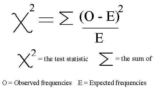
In our case: O1 = 10, O2 = 60, O3 = 30 & E1 = 50, E2 = 30, E3 = 20
Substituting the respective values in the above formula will give us an X-Squared value of 67.
Step 3 : Compare your X-Squared value with the critical value for the respective degree of freedom:
Let me first quickly explain the meaning of all the jargon in the above statement:
Degree of Freedom: The degree of freedom in this case is your total number of categories minus one. In our case, the total number of categories is 3 (Sprite, Coke, and Pepsi) which makes our Degree of Freedom or df = 2.
Critical Value: Go to the critical values table and find the critical value for df = 2 in the 0.05 probability column. Why 0.05 column? Well, there is a long explanation for that which'll take ages. Let's skip for now. Searching the table for the given parameters yields c = 5.991. The last thing to do is to compare the critical value with your X-Squared Value. If your X-Squared value is greater than the critical value then your observed values are too different from your expected values for the initial hypothesis to hold true in the current context and vice versa.
In our case since our X-Squared Value, 67 is greater than the critical value, 5.991 therefore we should not super impose the secondary research data on to the Waterloo Region's population with confidence. The Waterloo Region data is different enough that it deserves its own primary market research.